Goals and Background
Geoprocessing services are a relatively new frontier in the field of Web GIS. Geoprocessing services use many different spatial tools and inputs to solve GIS issues. For example, this lab demonstrates how to create geoprocessing serves over the web. This geoprocessing service will be created to determine the best potential locations to put a factory in Wisconsin. This is determined by filtering features. The factory location must be within a defined distance from rivers (minimum distance is 5 km), railroads (minimum distance is 5 km), location and a distance from that location (minimum is 50 km), and a defined population threshold for nearby cities (minimum is 4,000).
Methods
First, a new model was created with the work-space and scratch space environments set to a select file geodatabase. This model was created in a new Toolbox. The model created can be seen below in figure 5.0.
 |
| Fig 5.0: Model For Factory Sites |
There are four main input feature classes. These are the rivers, railroads, Wisconsin cities, and the input location of interest. The model starts with inputting a location of interest. This area of interest is a point which is specified when the model is ran. Then, a buffer from this point is created. This creates the Point_Buffer. Next, This Point_Buffer is clipped independently to the railroads feature class, rivers feature class and the selected cities feature class. The select tool on the cities to select cities which have a population of at least 4000. Next, a buffer is created from the railroads clip. Here, the input distance from these railroads is defined by the user. The minimum distance is 5 km. Similarly a buffer is created for the rivers also specified by the user. The minimum value is 5 km. Next, the city population threshold is specified by the end user, However, the minimum population is 4000. After that, the railroads buffer is intersected with the river buffer. Then, a spatial join is used to join the selected cities clip to the river and railroad buffer. The intersect tool is used here because using an intersect would result in the the output being a point geometry. The desired output is of the polygon geometry type. Also, the union tool wouldn't work because a union requires two polygon features; here, there is one polygon feature class and one point feature class. Lastly, the dissolve tool was used to eliminate internal boundaries within polygons. After the model was complete, it was ran, and the model was exported as a python script.
Next, this geoprocessing service was published to the development server. This was done by opening up the results window and then navigating to Share As → Geoprocessing Service. This was then published as an Asynchoronous service because the model will take several minutes to run. Once published, the service was published as a web map and then developed into a Web App using the Web AppBuilder Developer Edition. This was done using a similar process executed in lab 3. In the Web AppBuilder, the feature class symbology was changed so end users can easily understand the features. The geoprocessing widget was used to configure the labels for the model parameters. This is where the labels were made to be more user friendly. For example, "Input_DistanceToRailroads" was "Enter distance to railroads". The last step was to save the widget and test the model in the Web AppBuilder. This was done by clicking on the geoprocessing widget, placing an area of interest point on the map, entering the distance of interest, distance to railroads, and distance to rivers.
Results
The result of methods section is a Web application which can be accessed here: Determining Potential Factory Locations in Wisconsin. Note, this link can only be accessed if one is connected to the University of Wisconsin Eau Claire's internet. Figure 5.1 is a short video which shows how the web app works. In the video, the inputs all left to all their defaults: 5 km from rivers, 5 km from railroads, 4000 population threshold, and 50 km area distance of interest. The location of interest is placed in Prescott Wisconsin. Then, the model is ran. After the model runs, it shows the locations for the best potential factory locations in the the green polygon areas. Each time the model is ran, the best potential areas will change because of difference in the potential values in the input parameters. This web app could be used
Fig 5.1: Video of How of to Factory WebApp
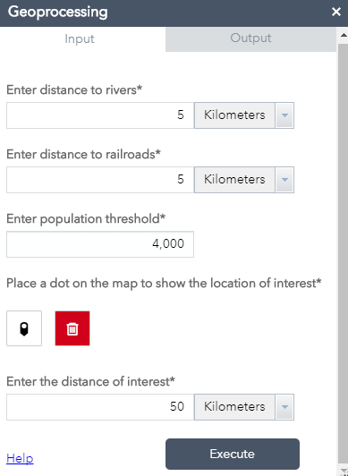
Figure 5.2 is a screenshot of what the interface looks like in the geoprocessing widget. This is where the end user can enter in the desired distance to rivers and railroads, population threshold, location of interest, and distance of interest. The default values can be changed to larger values by the end user.
 |
| Fig 5.2: Geoprocessing Widget Interface |
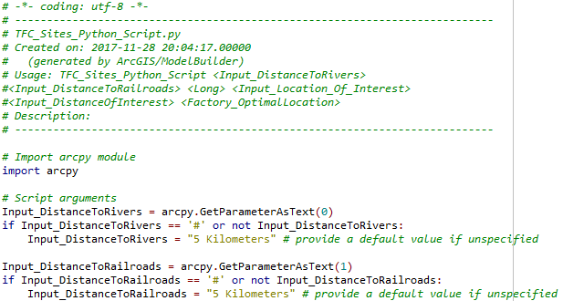
Also as part of the results is the python script generated when exporting the model to python. This script can be viewed here: Factory Model Python Script. If this script were to be ran in PyScripter, it would produce the same result as running the model in ArcMap. a screenshot of the first part of the python script is shown below in figure 5.3. Note that this python script could be used, but was not used in the creation of the geoprocessing service hence the script is a result and not a method.
 |
| Fig 5.3: Exported Python Script |
Sources
nhd.usgs.gov 2017, (n.d) Rivers Feature Class retrived from https://nhd.usgs.gov/
U.S. National Atlas, 2017. Wisconsin_Cities Feature Class
U.S. National Transportation Atlas, 2017. Railroads Feature Class
Wilson, C (2017) Lab 8 Geoprocessing Services Web App retrieved from
No comments:
Post a Comment